Demand Modeling

UCSD MGT 100 Week 04

Kenneth C. Wilbur and Dan Yavorsky

Let’s reflect

• Train (2009), Sec. 3.1, 3.3, 3.9
• Causal inference in econ and marketing by Varian

• I like the overview of modeling in the R4DS chapter. Basically a model of modeling
• We’ll talk about the Train content throughout, and the Varian content in the context of price endogeneity
• I hope you did the reading this week. If not, you may have some trouble keeping up, and you should probably consider doing the reading after class.

Demand Curves

• Theory
• Challenges
• What firms do

Inverse Demand Curve

• What’s this? why do we call it inverse?
• How would a company use this?
• Has anybody worked for a company?
• What was the company’s demand curve?
• does anybody have a parent or a sibling or a friend who works for a company?
• What was that company’s demand curve?
• has anybody ever heard a company CEO or employee talk about what their demand curve was?
• Have you heard anybody ask these questions before? Why not?

Demand Curves: Theory

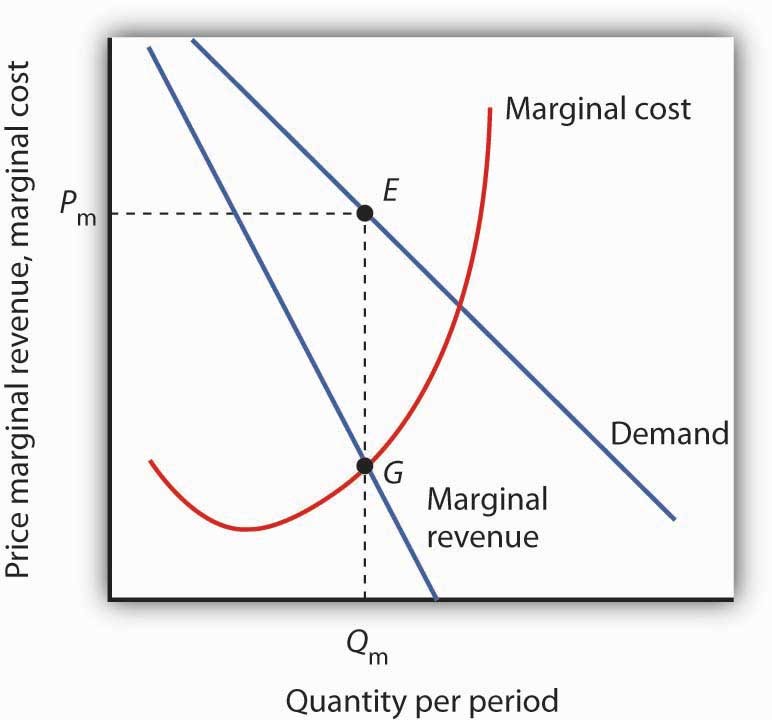
• Useful theoretical concept that summarizes market response to price

    - Why is it useful? 

• Often taught with perfect competition

    - Typically assumes stable, competitive, frictionless markets w free entry, full information, no differentiation 
    - Model predicts zero LR economic profits
    - Any evidence?

• Also, taught with monopoly i.e. market power

    - What is market power? How would we measure it?

• why useful? it lets you make counterfactual predictions. (what predictions?)
• No differentiation? What markets have no differentiation? Commodities… maybe? Stock market?
• what does competitive mean exactly? how do we measure it?
• intellectual property rights, company capabilities, consumer information sets all limit direct competition in most markets

Demand Curves: Challenges

• Idealized demand curves are hard to estimate (why?)

• Where do product attributes come in?

• Many things can predict demand

    - preferences, information, advertising, quality, match value, costs, complements, substitutes, competitor prices, entry, policy, taxes, retail distribution, nature of equilibrium, stockpiling, other consumer behaviors...

• What do we need to estimate Demand?

• We’re going to need a model and exogenous price variation to estimate demand

How firms learn demand

• Market research

      - Typically, conjoint analysis, customer interviews or simulated purchase environments 

• Expert judgments, e.g. salesforce input

• Cost-driven price adjustments

• Demand modeling with archival data

• Price experiments

    - Typically, market tests, digital experiments, bandits, coupons or other targeted price promotions

• Best practice: triangulation

• In many markets, costs can drive prices up, but they seldom drive them down
• If we disregard reactance and dynamics (stockpiling, reference prices, competitors), experiments are the single best way to learn demand, e.g. dube & misra (2019)

Price Experiments

• Ideally, the best way to learn demand, because you create exogenous price variation; but…

  • Competitors & consumers can observe price variation

  • May change purchase timing, stockpiling or
    reference prices

  • Competitors, distribution partners or suppliers may react

• Hence, experimenting to learn demand may change future demand

Demand Modeling: Pros

• Relatively inexpensive for large organizations

• Confidential

• Depends on real consumer choices, i.e. revealed preferences

• Enables counterfactual demand predictions at unobserved prices

• Enables predictions of competitor pricing response

• Evaluable after price changes or competitor price changes

Demand Modeling: Cons

• Requires data, exogenous price variation, time, effort, training, commitment, trust, organizational buy-in

• Always subject to untestable modeling assumptions

• Requires the near future to resemble the recent past

      - To be fair, all predictive analytic techniques require these 3

• Data and variation are distinct; e.g. if price never changed, good luck estimating demand
• what does exogenous mean? We’ll talk about that more later
• corr(future, past): Your estimated demand curve might become unreliable just when you need it the most
• Hence most often used in mature, stable markets; not so much in startups
• If you don’t know what you’re doing, you can pay a nearly infinite amount for the service
• If you do it wrong, it may range from useless to badly misleading (would you know?)

Do Demand Models Work?

• Evidence is scarce but supportive

  - Informally, I know several people who maintain demand models in large orgs
  - Formal evidence requires researchers and firm to collaboratively (a) estimate demand, (b) act on demand estimates, (c) observe how actions affect outcomes, & (d) report the results publicly. Hard to do & incentives conflict
  - Demand modeling can also go badly, e.g. due to price endogeneity

  • Misra & Nair (2011) : B2B sales & salesforce compensation

  • Nair et al. (2017) : Casino loyalty rewards

  • Pathak and Shi (2021) : School choice

  • Dube and Misra (2023) : ZipRecruiter ad pricing

Multinomial Logit

• history, math, discussion

Multinomial Logit (MNL)

• Old, famous, popular demand model
• Ported to econ from stats & psych by McFadden (1974, 1978, 1981; “Logistic regression’’)

• McFadden was an economist working to empiricize theoretical models of individual choice
• In early 1970s, he was funded by NSF to predict how BART would change transit in SF
• He organized a team that collected pre-BART transportations choices by commuters in neighborhoods that were to receive BART stations. Product attributes included things like walking distance, waiting time, financial cost, and automotive preference dummy
• He estimated a MNL using pre-BART individual level survey data, then simulated how transit choices would change after BART began operation
• This table shows how his predictions mapped onto the post-BART choices: he pretty much nailed his BART ridership predictions
• This stood in contrast to survey-based results, which predicted much larger BART ridership
• High-profile early “win” for MNL, combined with theoretical interpretation, led to model adoption

• Source: McFadden (1974)

Multinomial Logit (MNL)

• Let \(i\) index consumers, \(j=1,...,J\) products, and \(t\) index choice occasions

• Assume each \(i\) gets indirect utility \(u_{ijt}\) from product \(j\) in market \(t\):

\[u_{ijt}=x_{jt}\beta-\alpha p_{jt}+\epsilon_{ijt}\]

• Then, assuming each \(i\) picks the \(j\) that maximizes \(u_{ijt}\), has unit demand, and that \(\epsilon_{ijt}\sim\)i.i.d.\(EV_1(0,1)\), market share is

\[Prob.\{u_{ijt}>u_{ikt}\forall{k\ne j}\}\equiv s_{jt}=\frac{e^{x_{jt}\beta-\alpha p_{jt}}}{\sum_{k=1}^J e^{x_{kt}\beta-\alpha p_{kt}}}\]

With \(N_t\) consumers, \(q_{jt}(\vec{x}; \vec{p})=N_t s_{jt}\). See Train 2009 sec 3.10 for proof

• Estimating \(\alpha\) and \(\beta\) enables us to predict every product’s quantity response to a change in any product’s attributes \(x_{jt}\) or price \(p_{jt}\)

• AKA multinomial logistic regression
• t could be repeated observations of a single market, multiple distinct markets at the same time, or both
• We obtain the market share formula by integrating the likelihood of u_ijt exceeding all other u_ikt’s, over the space of the epsilons and the i’s
• the reason we assume iid EV(0,1) is bc it gives us this nice tractable expression with useful properties
• s_jt is bounded by 0 and 1

MNL: Common factors

• Suppose \(\gamma_{t}\) indicates how popular the category is in market \(t\), so utility is \(u_{ijt}=\gamma_{t}+x_{jt}\beta-\alpha p_{jt}+\epsilon_{ijt}\). Then market share becomes

\[s_{jt}=\frac{e^{\gamma_{t}+x_{jt}\beta-\alpha p_{jt}}}{\sum_{k=1}^J e^{\gamma_{t}+x_{kt}\beta-\alpha p_{kt}}}\]

\[s_{jt}=\frac{e^{\gamma_{t}} e^{x_{jt}\beta-\alpha p_{jt}}}{e^{\gamma_{t}}\sum_{k=1}^J e^{x_{kt}\beta-\alpha p_{kt}}}\]

\[s_{jt}=\frac{e^{x_{jt}\beta-\alpha p_{jt}}}{\sum_{k=1}^J e^{x_{kt}\beta-\alpha p_{kt}}}\]

• Similar exercise applies to individual-specific intercepts \(\gamma_i\), or individual-time interactions \(\gamma_{it}\). Only differences across products affect predicted market shares

• Hence any factor that doesn’t vary across products will drop out of the model

MNL: Share differences

• We set product \(j=1\) utility to \(u_{i1t}=\epsilon_{i1t}\) to normalize utility, i.e.

\[s_{1t}=\frac{1}{\sum_{k=1}^J e^{x_{kt}\beta-\alpha p_{kt}}}\]

• Hence for every \(j\ne 1\), consider an affine transformation of market shares:

\[ln(s_{jt})-ln(s_{1t})=x_{jt}\beta-\alpha p_{jt}\]

• Looks like a regression equation… we sometimes add an error \(\xi_{jt}\) to represent unobserved product attributes:

\[ln(s_{jt})-ln(s_{1t})=x_{jt}\beta-\alpha p_{jt}+\xi_{jt}\]

• It’s the \((J-1)T\) differences in market shares that identify demand parameters

• Often, we normalize the non-purchase option which has no attributes, and call it the “outside option”

MNL Estimation

Define \(y_{ijt} \equiv 1\{i \text{ chose } j \text{ in } t\}\). I.e., \(y_{ijt}=1\) iff \(i\) choose \(j\) at \(t\); otherwise \(y_{ijt}=0\).

1. Maximum likelihood: Assume the probability of observation \(\{i,j,t\}\) is \(s_{jt}^{y_{ijt}}\);
   then lik. is \(L(\beta )=\prod\limits_{\forall i,j,t} s_{jt}^{y_{ijt}}\); & choose parameters to maximize log lik:

\[\sum_{\forall i,j,t} y_{ijt}\ln s_{jt}\]

2. Method of Moments: Choose \(\alpha\) and \(\beta\) to solve some vector of “moments,” i.e. interactions between observables \(z\) and error terms, e.g. 

\[ \sum_{\forall j,t}z_{jt} (\frac{\sum_{\forall i}y_{ijt}}{N_t} - s_{jt})=0\]

3. Linearize the model and choose parameters to minimize the sum of square errors

MNL Goodness-of-fit Statistics

• Discrete choice models predict choice probabilities rather than choices, because utility is always unobserved; hence nonstandard fit statistics

• Predicted outcomes are inherently stochastic, so limited predictive ability

1. Likelihood Ratio Test: (not R-sq)

\[\rho=1-\frac{ln L(\hat\beta)}{ln L(0)}\]

• As \(L(\hat\beta)\to 1\), \(ln L(\hat\beta)\to 0\), \(\rho\to 1\)

• As \(ln L(\hat\beta)\to ln L(0)\), \(\rho\to 0\)

      -   Heuristic: 0.2-0.4 is pretty good

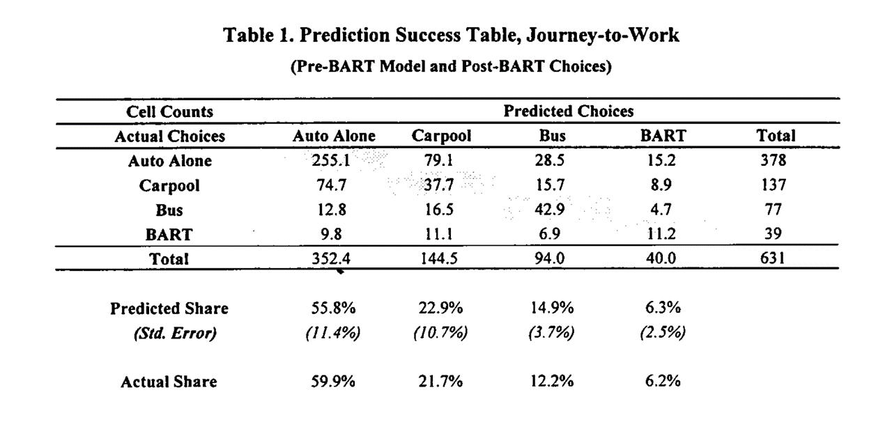
2. Hit Rate: % of individuals for whom most-probable choice was actually chosen

3. R-sq using prediction errors at the \(jt\) level

• #3 is appealing idea but based on fewer data points than estimation

MNL Pros

1. Microfounded, i.e. behavioral predictions are consistent with a clearly specified theory of consumer choice

      - Economists widely believe that microfounded models are more generalizable than purely statistical models*

2. Extensions accommodate preference heterogeneity

     - We'll cover 3 types of extensions when we cover heterogeneous demand modeling

3. Likelihood function is globally concave in the parameters, ensuring fast and reliable estimation

*This paper supports this belief

MNL Cons

1. Assuming \(\epsilon_{ijt}\sim\)i.i.d.\(EV_1(0,1)\) is convenient but unrealistic

    - Alternatives exist but can be computationally expensive

2. Analyst selects the choice set \(J\), market size \(N_t\), attributes \(x_{jt}\), and price structure \(p_{jt}\).

    - What's a j? What's a t? What's in x? How do we measure p? Who's in N?

3. Market share derivatives depend on market shares alone (IIA; see Train Sec. 3.6)

4. Price Endogeneity

      - Affects all demand models

• Unobservables would likely be correlated across people, products and markets
• We would expect more-differentiated products to face less-elastic demand, holding market shares constant
• Derivatives statement presented without proof, refer interested students to the chapter. Some people think this property is appealingly simple, but it would be more realistic if the derivatives depended on the attribute levels or prices directly

IIA: Deeper dive

• Famous example from McFadden (1974)
• Suppose you estimate demand for transportation with three options: {Blue Bus, Red Bus, Car}, each with 33% market share
• Now suppose you painted the red buses blue and want to predict market shares in the new choice set: {Blue Bus, Car}
• MNL will predict Blue Bus and Car shares of 50%, not 67% and 33% (why?)

IIA: Remedies

IIA is testable & usually rejected by data

3 common remedies:

1. Impose structure on choice set,
   e.g. Nested Logit or Ordered Logit

2. Relax i.i.d. assumption, e.g. Multivariate Probit

3. Change model structure so IIA does not hold, e.g. heterogeneous logit

Price endogeneity

• Fundamental issue: Demand model should be a causal relationship but prices are usually nonrandom. We have to distinguish correlation from causation

      - Prices may covary with unobserved demand shifters, unmeasured product attributes or other missing variables
      - Price endogeneity is a measurement problem, not a modelling problem
      - Hard to verify empirically--needed data is missing--but widely believed important

• \(\hat{\alpha}\) will be biased when prices depend on unmodeled demand factors (e.g., image, reliability). Implies wrong demand slope, biased demand predictions

• Typically, bias will be toward zero (“too flat”), hence underestimating price sensitivity and overestimating price change

• Affects all demand models, not just MNL

• Common solutions: Experiments or quasi-experiments (Instrumental variables, regression discontinuities, natural experiments, dfce-in-dfce, synthetic control, double/debiased machine learning)

Price endogeneity in MNL

• Berry (1994): Linearize MNL and use instruments

\(ln(s_{jt})-ln(s_{1t})=x_{jt}\beta-\alpha p_{jt}+\xi_{jt}\)

• Valid instruments will (1) predict \(p_{jt}\) and (2) don’t predict \(\xi_{jt}\)

        (1) is testable; (2) is not
        Classic instruments are input prices

• In general price endogeneity requires careful attention

   - We set up our smartphone sales data with exogenous price variation in promotions, so this class will disregard it for simplicity
   - Price endogeneity leads to biased demand slope, which could lead to biased price recommendation, which could lead to suboptimal outcomes
   - Endogeneity is a major topic in graduate study

• We’re just naming it for you here, so you don’t get surprised if someone else tells you about it. When demand modeling disagrees with price experiments, endogeneity is a likely culprit. It’s important, but we could easily spend the rest of the quarter on this topic, and we would rather spend the time on what we can do with models.
• Your standard advice to a firm would be to induce nonobvious experimental variation when possible in order to estimate price responsiveness, such as price variation across markets or targeted coupons
• Price response tends to be pretty strong so you don’t necessarily need a big intervention

• T/F: The MNL assumes all consumers have the same preference parameters.

Class script

• Wrangle data
• Estimate MNL
• Interpret parameters and SEs
• Assess model fit

Wrapping up

Homework

• Let’s take a look

Recap

• Demand modeling enables data-driven sales predictions for counterfactual prices and attributes
• MNL is popular bc it is powerful, microfounded and tractable
• MNL has some important limitations (eg, IIA) which can be alleviated by modeling heterogeneity
• Price endogeneity is a measurement problem that biases demand parameter estimates when price is correlated with unobserved demand shifters. Can often be resolved through experimental or quasi-experimental techniques

Going further

• Causal inference as a blind spot of data scientists

• McFadden’s Nobel Lecture

• Discrete Choice Analysis with R

• Microeconometric models of consumer demand by Dube

• Empirical Models of Demand and Supply in Differentiated Products Industries by Gandhi & Nevo

• Personalized Pricing and Customer Welfare by Dube & Misra

• The McFadden lecture will give further historical and theoretical context to MNL and its extensions
• Varian (2016) covers causal inference in marketing
• Dube (2019) surveys the literature on demand modeling
• Gandhi & Nevo survey demand modeling & consider it simultaneously with supply modeling
• Misra & Dube (2021) ran a price experiment with ZipRecruiter, used a demand model to price-discriminate among job recruiters, and then report the results of implementing the personalized prices. Profits went up by about 80%, with about 60% of that coming from optimizing the overall price