Heterogeneous Demand

UCSD MGT 100 Week 06

Kenneth C. Wilbur and Dan Yavorsky

Let’s reflect

• Train (2009), Sec. 6.1, 6.2, 6.8

• The Train chapter gives a good background to much of today’s technical material, in the specific context of the MNL with heterogeneity
• the r4ds chapter is more general in terms of model building, and relates to what we’ll do in the script, as we have to decide what to include in x and w

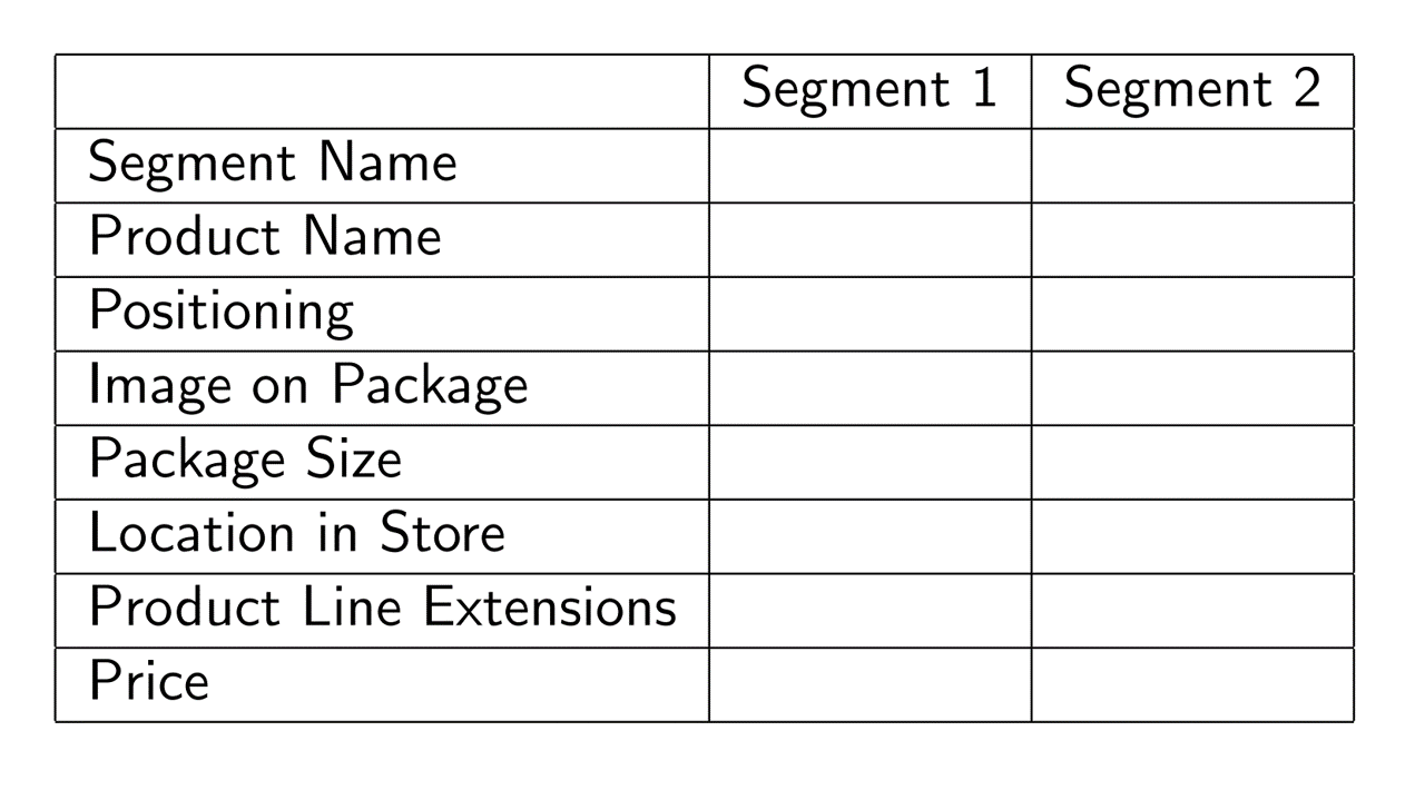
Segmentation Case study: Quidel

• Leading B2B manufacturer of home pregnancy tests
• Tests were quick and reliable
• Wanted to enter the B2C HPT market
• Market research found 2 segments of equal size;
  what were they?

• How did price sensitivity differ between the two segments?

• Google Pixel Ad

• Source
• Key learning here: Understanding how customer preferences differ between segments can enable optimization of product attributes for specific segments
• In this case, because most smartphone users never change the default camera settings, the default settings were optimized given local preferences, leading to a 48% market share for transsion
• The Google ad suggests that Google is also figuring out some of the same heterogeneous preferences for smartphone camera attributes, and how tuning defaults for local markets might increase sales

Het. Demand Models

1. Discrete heterogeneity by segment

2. Continuous heterogeneity by customer attributes

3. Individual-level demand parameters

          -   We'll do 1 & 2

• Multiple approaches can be used together

MNL Demand

• Recall our MNL market share function \(s_{jt}=\frac{e^{x_{jt}\beta-\alpha p_{jt}}}{\sum_{k=1}^{J}{e^{x_{kt}\beta-\alpha p_{kt}}}}\)

• What is \(\alpha\)?

• What is \(\beta\)?

• What limitations does this model have?

• Incorporating customer heterogeneity into demand models can enable a rich array of segment-specific or person-specific customer analytics

• Everything here is review; please ask about anything unclear
• By construction, base model assumes away the possibilities that (i) preference parameters vary across customer segments, or (ii) covary with customer attributes, or (iii) differ across customers at all. So we’ve ruled out the existence of hopefuls and fearfuls
• where are the hopefuls and fearfuls?

Why add het.?

1. MNL can estimate quality; Het demand estimates quality & fit

2. Better “policy experiments” for variables we {manage,can measure,predict sales}

      - Pricing: price discrimination, two-part tariffs, fees, targeted coupons
      - Customer relationships: Loyalty bonus, referral bonus, freebies
      - Social media: Posts, likes, shares, comments, reviews
      - Advertising: Ad frequency, content, media, channels
      - Product attributes: Targeted attributes, line extensions, brand extensions
      - Distribution: Partner selection, intensity/shelfspace, exclusion, in-store environment

3. Predicts M&A results; oft used in antitrust

• Demand models let us estimate product qualities, but not product fit
• Heterogeneous demand models enable measurement of both vertical & horizontal dimensions of product differentiation

1. Discrete heterogeneity by segment

• Assume each customer \(i=1,...,N\) is in exactly 1 of \(l=1,...,L\) segments with sizes \(N_l\) and \(N=\sum_{l=1}^{L}N_l\)
• Assume preferences are homogeneous within segments, and heterogeneous between segments
• Replace \(u_{ijt}=x_{jt}\beta-\alpha p_{jt}+\epsilon_{ijt}\) with \(u_{ijt}=x_{jt}\beta_l-\alpha_l p_{jt}+\epsilon_{ijt}\)
• That implies \(s_{ljt}=\frac{e^{x_{jt}\beta_l-\alpha_l p_{jt}}}{\sum_{k=1}^{J}e^{x_{kt}\beta_l-\alpha_l p_{kt}}}\) and \(s_{jt}=\sum_{l=1}^{L}N_l s_{ljt}\)
• We will do this with predefined segments based on usage
• We can also estimate segment memberships. Pros and cons?

• Pro: don’t have to define the segment memberships ex ante
• Cons: noisy; may be inconsistent over time; demanding of the data; ignores available theory; possible numerical issues
• Kamakura & Russell (1989)

2. Continuous heterogeneity by customer attributes

• Let \(w_{it}\sim F(w_{it})\) be observed customer attributes that drive demand, e.g. usage

• \(w_{it}\) is often a vector of customer attributes including an intercept

• Assume \(\alpha=\gamma w_{it}\) and \(\beta=\delta w_{it}\)

• Then \(u_{ijt}=x_{jt}\delta w_{it}- p_{jt}\gamma w_{it} +\epsilon_{ijt}\) and

\[s_{jt}=\int \frac{e^{x_{jt}\delta w_{it}- p_{jt}\gamma w_{it}}}{\sum_{k=1}^{J}e^{x_{jt}\delta w_{it}- p_{jt}\gamma w_{it}}} dF(w_{it}) \approx \frac{1}{N_t}\sum_i \frac{e^{x_{jt}\delta w_{it}- p_{jt}\gamma w_{it}}}{\sum_{k=1}^{J}e^{x_{jt}\delta w_{it}- p_{jt}\gamma w_{it}}}\]

      - We usually approximate this integral with a Riemann sum

• What goes into \(w_{it}\)?

• What if \(dim(x)\) or \(dim(w)\) is large?

• We could use theory to restrict elements of \(\gamma\) and \(\delta\) to 0
• We could use PCA to project x or w onto a lower-dimensional space
• We could use Lasso, Ridge, Elastic Net, etc. for data-driven parsimony
• Riemann sums
• Goettler & Shachar (2001)

3. Individual demand parameters

• Assume \((\alpha_i,\beta_i)\sim F(\Theta)\)

      - Includes the Hierarchical Bayesian Logit from weeks 2&3

• Then \(s_{jt}=\int\frac{e^{x_{jt}\alpha_i-\beta_i p_{jt}}}{\sum_{k=1}^{J}e^{x_{jt}\alpha_i-\beta_i p_{jt}}}dF(\Theta)\)

• Typically, we assume \(F(\Theta)\) is multivariate normal, for convenience, and estimate \(\Theta\)

  • We usually have to approximate the integral, often use Bayesian techniques (MSBA/PhD)
  • Or, we can estimate \(F\) but that is very data intensive
  • In theory, we can estimate all \((\alpha_i,\beta_i)\) pairs without \(\sim F(\Theta)\) assumption, but requires numerous observations & sufficient variation for each \(i\)

• The Bayesian estimation techniques are compute intensive and usually require MCMC sampling; see MSBA

How to choose?

• Humans choose the model

• How do you know if you specified the right model?

      - Hints: No model is ever "correct." No assumption is ever "true" (why not?)

• How do you choose among plausible specifications?

• Pros and cons of model enrichments or simplifications?

• All models are wrong. Some models are useful

• Should you model weight=f(height) or height=f(weight)?
• Notice the many:1 correspondence of weight to height, may make prediction difficult
• notice the discrete nature of height measurements
• consider the theoretical relationship
• Does it matter whether height is measured in inches (adults) or centimeters (babies)?
• Ultimately it depends on your purpose. “All models are wrong, some models are useful”
• Considerations: Theory; Modeling objective; Precision; Causal ordering

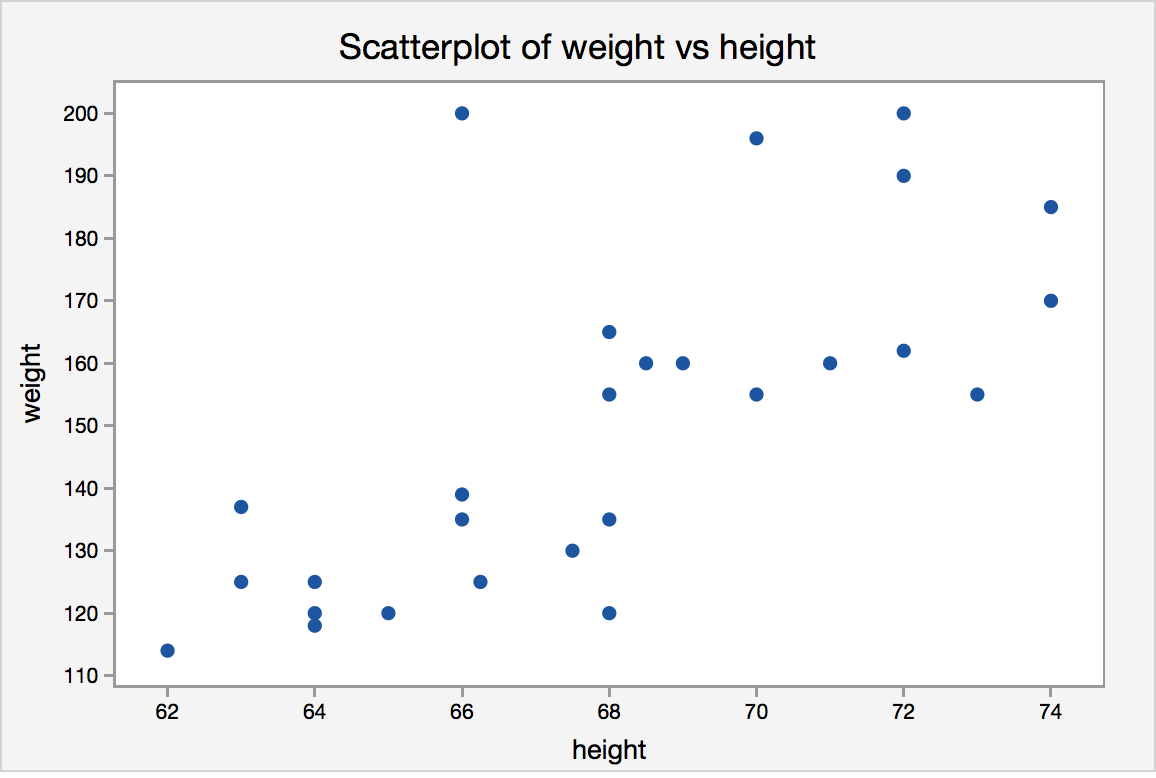
Model specification

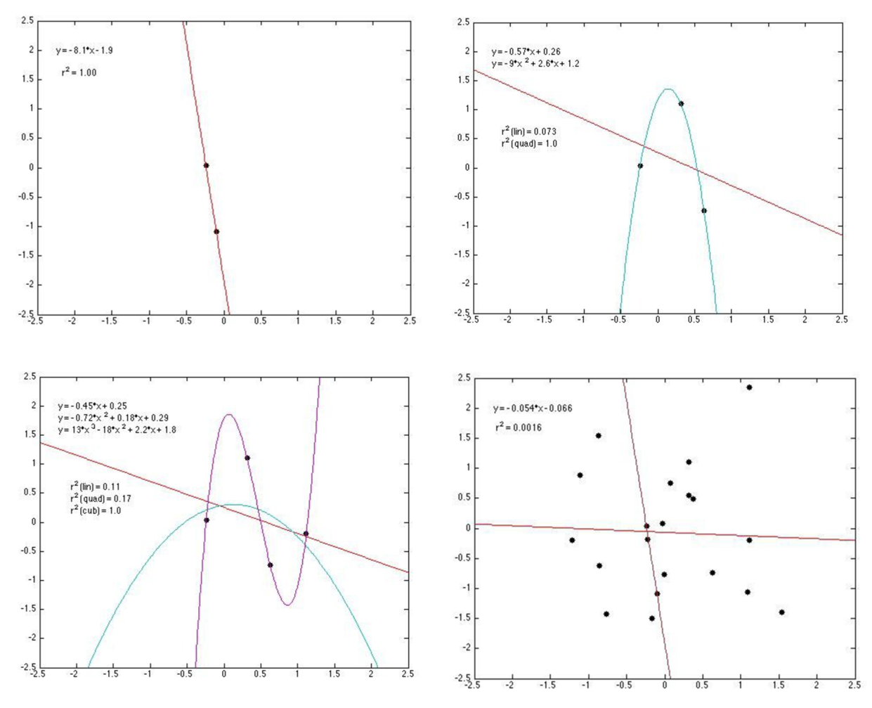
• Bias-variance tradeoff

    - Adding predictors always increases model fit
    - Yet parsimony often improves predictions

• Many criteria drive model selection

    - Modeling objectives
    - Theoretical properties
    - Model flexibility 
    - Precedents & prior beliefs
    - In-sample fit
    - Prediction quality
    - Computational properties

• Here we want to visualize the process of overfitting
• Let’s imagine you’re estimating demand at a B2B firm with few customers
• Suppose you had 2 data points. You standardize your variables and fit a line. R2 = 1 !!
• Then you get another data point. You standardize again and fit a quadratic. R2 = 1 !!
• Then you get a 4th data point. Standardize again & fit a cubic. R2 = 1 undefeated
• … you see the problem here? … consider # of degrees of freedom & # of parameters
• Finally, suppose you had lots of data as in lower-right. Then you might discover the relationship is actually quite weak, and you have been dramatically overestimating the strength of the relationship up until now
• Is the true relationship actually changing with your sample size? Or are you just getting more data points?
• Source
• Another example: Suppose you studied for an exam by memorizing every word of the textbook. Then the professor asked you questions that asked you to apply your understanding of the text. If the only thing you did was return the text contents, you would get the questions wrong. That would be overfitting.

How to avoid overfitting?

• Retrodiction = “RETROspective preDICTION”

        - Knowing what happened enables you to evaluate prediction quality
        - We can compare different models and different specifications on retrodictions

• We can even train a model to maximize retrodiction quality (“Cross-validation”)

        - Most helpful when the model's purpose is prediction
        - More approaches: Choose intentionally simple models
        - Penalize the model for uninformative parameters: Lasso, Ridge, Elastic Net, etc.

Cross-validation

• Exercise to evaluate retrodiction performance and reduce overfitting risk among a set of candidate models \(m=1,...,M\). Algorithm:

1. Randomly divide the data into \(K\) distinct folds
2. Hold out fold \(k\), use remaining data to estimate model \(m\), make predictions for fold \(k\); store prediction errors
3. Repeat 2 for each \(k\)
4. Repeat 2&3 for every model \(m\)
5. Retain the model with minimum prediction errors

• We often learn that most reasonable models perform similarly
• It’s really important to keep in mind that cross-validation is simply 1 input into the model selection criterion. It will matter most when our main objective is prediction. Even then it won’t be the sole model selection criterion

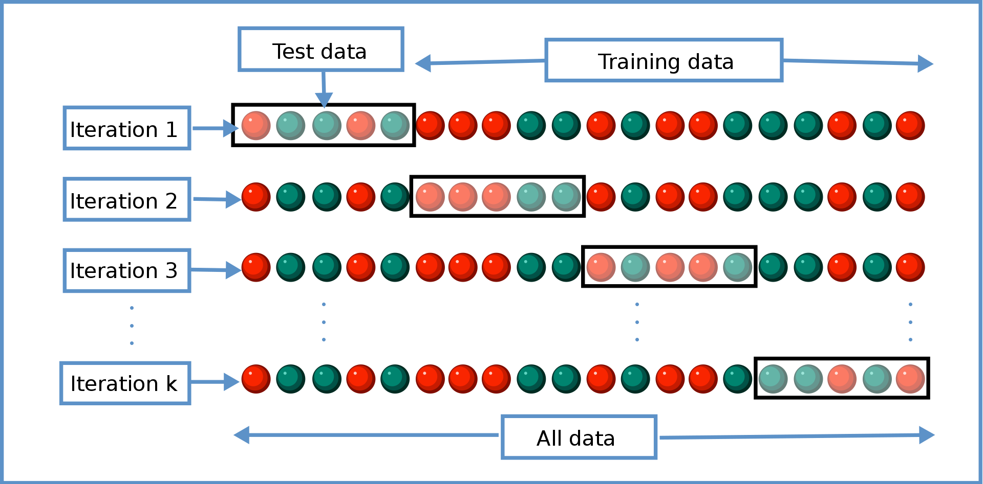
        - You estimate the model K times
        - Each estimation uses a different (K-1)/K proportion of the data
        - We evaluate retrodiction quality K times, then average them
        - When K=N, we call that "leave-one-out" cross-validation
        - Important: cross-validation is just one tool in the toolbox
        - Final model selection also depends on theory, objectives, other criteria

Ex-post evaluations

• Can a model withstand changes in the environment?
• Non-random holdouts are strong tests, but can only be retrospective

• Source

Het demand modeling: More considerations

• Customer data needs to be high quality (GIGO, Errors-in-variables biases)
• Implementation needs to consider qualitative factors {effectiveness, legality, morality, privacy, conspicuousness, equity, reactance, costs, speed, understanding}
  • Guiding principle (not a rule):
    Using data to legally, genuinely serve customers’ interests is usually OK
  • Using private data against customer interest can harm some consumers, break laws, or incur liability. Litigation can kill a start-up
  • Major US laws: COPPA, GLBA, HIPAA, patchwork of state laws
• Heterogeneity in a demand model does not resolve price endogeneity

• garbage in, garbage out

• T/F: Adding random predictors into \(X\) can decrease OLS \(R^2\).

Class script

• Add heterogeneity to MNL model
• Individual-level heterogeneity via price-minutes interaction
• Segment-level heterogeneity via segment-attribute interactions
• Both

Wrapping up

Homework

• Let’s take a look

Recap

• Heterogeneous demand models enable personalized and segment-specific policy experiments

• Demand models can incorporate discrete, continuous and/or individual-level heterogeneity structures

• Heterogeneous models fit better, but will predict worse if overfit

Going further

• Heterogeneity in more detail

• Train (2009), Chapters 7-12

• Reconciling modern machine learning practice and the bias-variance trade-off