Heterogeneous Demand Modeling
MGT 100 Week 5
This version: May 2026 | License: CC BY 4.0 | We use javascript to track readership.
We welcome reuse with attribution. Please share widely.
Segmentation Case Study: Quidel
- Leading B2B manufacturer of home pregnancy tests
- Tests were quick and reliable
- Wanted to enter the B2C HPT market
- Market research found 2 segments of equal size;
what were they?
Hint: Both segments were about the same size, and both had very similar distributions of customer demographics
| Segment 1 | Segment 2 | |
|---|---|---|
| Segment Name | ||
| Product Name | ||
| Positioning | ||
| Image on Package | ||
| Package Size | ||
| Location in Store | ||
| Product Line Extensions | ||
| Price |
What does this heterogeneity distribution imply for relevant strategic choices?
![]()
A phone shopper first snaps a photo and examines the result. How might the photo quality influence their perception of the phone’s less evaluable features?
Digital Default Frequencies
- Classic study: 95% of MS Word users maintained original default options
- Classic study: 81-90% of users don’t use Ctrl+F
- Classic study: Randomizing top 2 search results only changed click rates from 42%/8% to 34%/12%
- 2021 data: Safari has 90% share on iPhone, Chrome (74%) and Samsung Internet (15%) have 89% share on Android
- Chrome always preinstalled on Android, Samsung Internet preinstalled on 58% of Android devices
- Why? Defaults are good enough; changing is hard, uncertain; users assume designer knows best; popularity implies utility; possible fear of norm deviation
Figures show the importance of understanding digital user needs, rather than assuming that usage indicates satisfaction
Het. Demand Models
- Heterogeneity by customer attributes
- Heterogeneity by segment
- Individual-level demand parameters
- We’ll code 1 & 2
- 3 is often best but needs advanced techniques → graduate study
MNL Demand
- Recall our MNL market share function \(s_{jt}=\frac{e^{x_{jt}\beta-\alpha p_{jt}}}{\sum_{k=1}^{J}{e^{x_{kt}\beta-\alpha p_{kt}}}}\)
- Recall that the model can predict how much any change in any product’s x or p would affect all products’ market shares
- What is \(\alpha\)? What is \(\beta\)?
- What are the model’s main limitations?
- Assumes all customers have the same attribute preferences
- Assumes all customers have same price sensitivity
- IIA: Predictions become unreliable when choice sets change
- Requires exogenous price variation to estimate \(\alpha\) (all demand models)
- Assumes iid \(\epsilon\) distribution: Convenient but unrealistic
Modeling heterogeneity can alleviate the first 3 and enable better predictions, but not price endogeneity.
However, predictive performance will worsen if we overfit the model. Have you heard of cross-validation?
Mapping Heterogeneity Extensions

Analyst can impose heterogeneity assumptions or seek to learn heterogeneity structure from data (very demanding). Tradeoff depends on empirical reasonableness of modeling assumptions vs. data thickness/sparsity
Heterogeneity by Customer Attributes
- Let \(w_{it}\sim F(w_{it})\) be observed customer attributes, needs or behaviors that drive demand
- \(w_{it}\) is often a vector of customer attributes including an intercept
- Assume \(\beta=\delta w_{it}\) and \(\alpha=w_{it} \gamma\) :: \(\delta\) & \(\gamma\) conformable matrices
- Suppose \(x_{jt}\) is 1x5, and \(w_{it}\) is 2x1, then \(\delta\) would be 5x2
- Then \(u_{ijt}=x_{jt}\delta w_{it}- w_{it} \gamma p_{jt} +\epsilon_{ijt}\) and
\[s_{jt}=\int \frac{e^{x_{jt}\delta w_{it}- w_{it}\gamma p_{jt} }}{\sum_{k=1}^{J}e^{x_{kt}\delta w_{it}- w_{it}\gamma p_{kt} }} dF(w_{it}) \approx \frac{1}{N_t}\sum_i \frac{e^{x_{jt}\delta w_{it}- w_{it}\gamma p_{jt}}}{\sum_{k=1}^{J}e^{x_{kt}\delta w_{it}- w_{it}\gamma p_{kt}}}\]
- We usually approximate this integral with a Riemann sum
We often restrict elements in \(\delta\) and \(\beta\) to zero, if we think the interaction is unimportant, to avoid overparameterizing the model. What goes into \(w_{it}\)? What if \(dim(x)\) and/or \(dim(w)\) is large?
Heterogeneity by Segment
- Assume each customer \(i=1,...,N_t\) is in exactly 1 of \(l=1,...,L\) segments with sizes \(\sum_{l=1}^{L}N_{lt}=N_t\)
- We will use 3 kmeans segments based on 6 usage variables
- Assume preferences are uniform within segments & vary between segments
- Consistent with the definition of segments
- Replace \(u_{ijt}=x_{jt}\beta-\alpha p_{jt}+\epsilon_{ijt}\) with \(u_{ijt}=x_{jt}\beta_l-\alpha_l p_{jt}+\epsilon_{ijt}\)
- That implies \(s_{ljt}=\frac{e^{x_{jt}\beta_l-\alpha_l p_{jt}}}{\sum_{k=1}^{J}e^{x_{kt}\beta_l-\alpha_l p_{kt}}}\) and \(s_{jt}=\sum_{l=1}^{L}N_{lt} s_{ljt}\)
Alternatively, it is possible to estimate segment memberships, rather than supplying them via kmeans. Pros: We don’t have to pre-specify segment memberships. Cons: Noisy, so we need a lot of data to do this well.
Individual Heterogeneity
- Assume \((\alpha_i,\beta_i)\sim F(\Theta)\)
- Includes the Hierarchical Bayesian Logit
- Then \(s_{jt}=\int\frac{e^{x_{jt}\beta_i-\alpha_i p_{jt}}}{\sum_{k=1}^{J}e^{x_{kt}\beta_i-\alpha_i p_{kt}}}dF(\Theta)\)
- Typically, we assume \(F(\Theta)\) is multivariate normal, for convenience, and estimate \(\Theta\)
- We usually have to approximate the integral, often use Bayesian techniques (MSBA/PhD)
- Or, we can estimate every \(\alpha_i\) and \(\beta_i\), that is very very data intensive
- In theory, we can estimate all \((\alpha_i,\beta_i)\) pairs without \(\sim F(\Theta)\) assumption, but requires numerous observations & sufficient variation for each \(i\). Most data intensive
How to Choose?
- “All models are wrong. Some models are useful” (Box)
- “Truth is too complicated to allow anything but approximations.” (von Neumann)
- “The map is not the territory” (Box)
- “Scientists generally agree that no theory is 100% correct. Thus, the real test of knowledge is not truth, but utility” (Hariri)
- No model is ever “correct,” No assumption is ever “true” (why not?)
- Model selection: A Judgment Problem
- How do you choose among plausible specifications?
- Involves both model selection — which f() in y=f(x) — and predictor selection
Use modeling purposes and constraints as model selection criteria. Purposes can include prediction, explanation and decision-making. Constraints can include privacy and ethics. What criteria would you prioritize?
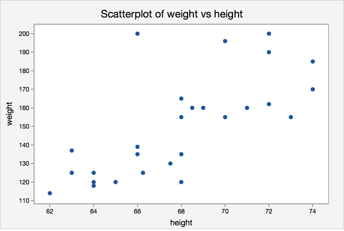
Should you model weight=f(height) or height=f(weight)? Notice the many-to-one correspondence and the discrete nature of height measurements.
Model Specification
- Bias-variance tradeoff
- Adding predictors always increases model fit
- Yet parsimony often improves predictions
- Many criteria drive model selection
- Modeling objectives
- Theoretical properties
- Model flexibility
- Precedents & prior beliefs
- In-sample fit
- Prediction quality
- Computational properties
Imagine you prepared for a quiz by perfectly memorizing the textbook but without understanding the material. Could you accurately apply the concepts in unseen settings?
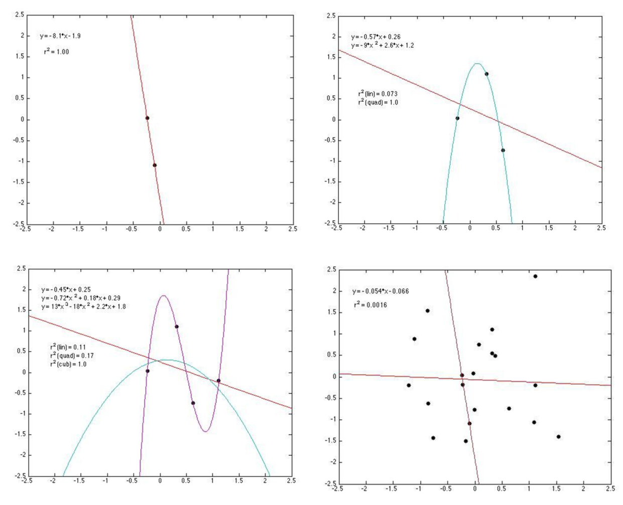
Choosing a model that maximizes a single criterion, such as R-square, can lead to bad decisions.
Regularization: Lasso, Ridge & Elastic Net
Adding predictors always improves in-sample fit but risks overfitting. Regularization methods penalize model complexity on the theory that simpler models predict better:
- Lasso (L1 penalty): \(\min_\beta \sum(y_i - x_i\beta)^2 + \lambda\sum|\beta_k|\)
- Can shrink coefficients to exactly zero → automatic variable selection
- Useful when only a few predictors matter
- Ridge (L2 penalty): \(\min_\beta \sum(y_i - x_i\beta)^2 + \lambda\sum\beta_k^2\)
- Shrinks all coefficients toward zero, but seldom to exactly zero
- Useful when many predictors each contribute small effects
- Elastic Net (L1 + L2): \(\min_\beta \sum(y_i - x_i\beta)^2 + \lambda_1\sum|\beta_k| + \lambda_2\sum\beta_k^2\)
- Combines Lasso and Ridge
The tuning parameter \(\lambda\) controls penalty strength: higher \(\lambda\) → more shrinkage, fewer effective parameters. Cross-validation is typically used to choose \(\lambda\).
If you have 100 product attributes but suspect only 10 matter, Lasso identifies which ones while Ridge keeps all 100 with smaller weights. Penalties are assumed as proxies for overfitting, but overfitting is not directly optimized.
How to Evaluate Overfitting?
- Retrodiction = “RETROspective preDICTION”
- Quantifies model’s ability to generalize to non-training data
- We can compare different models and different specifications on retrodictive accuracy
- We can even train a model to maximize retrodiction quality (“Cross-validation”)
- Most helpful when the model’s purpose is prediction
Be careful not to confuse retrodiction with prediction. Why not?
Cross-Validation Algorithm
- General approach to evaluate retrodiction performance and overfitting risk among a set of competing models \(m=1,...,M\). Algorithm:
- Randomly divide the data into \(K\) distinct folds
- Hold out fold \(k\), use remaining \(K-1\) folds to estimate model \(m\), then predict outcomes in fold \(k\); store prediction errors
- Repeat 2 for each \(k\)
- Repeat 2&3 for every model \(m\)
- Retain model \(m\) with minimal prediction errors, usually MAPE or MSPE
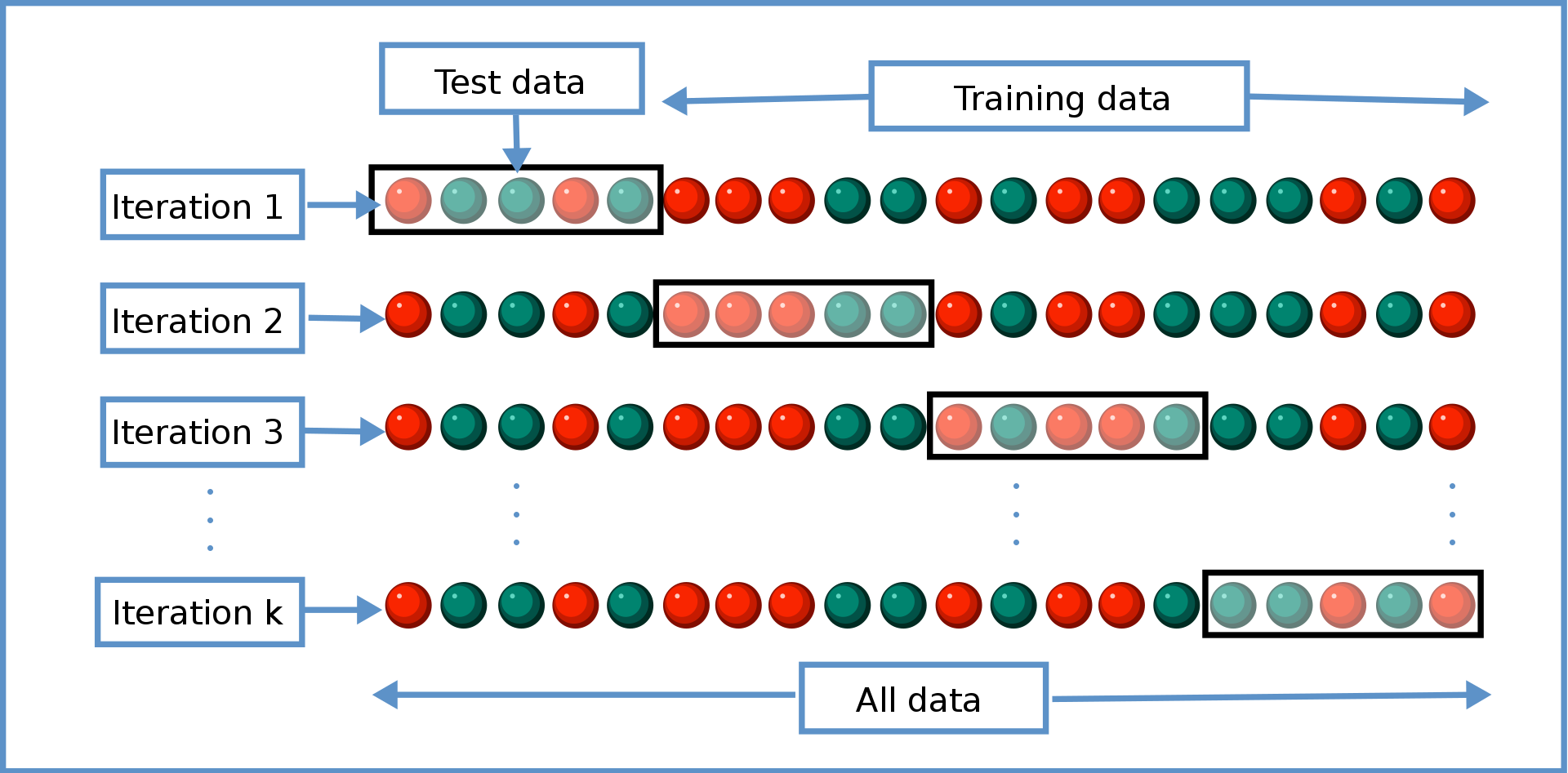
- You estimate every model K times (K=4 in the graphic); each uses a different (K-1)/K proportion of the data
- We evaluate each model’s retrodiction quality K times, then average them
- When K=N, we call that “leave-one-out” cross-validation
- Cross-validation is just one criterion; final model selection also depends on theory, objectives, other criteria
Non-Random Holdout Evaluations
- When are models most robust to major changes in the data-generating process?
- Non-random holdouts are strong tests, but can only be retrospective

This paper evaluated retrodictive performance of various models of auto production and pricing estimated using pre-2008 data after the 2008 gas price shock. It supported the generalizability of microfounded models. In what scenarios are tests like this most valuable?
Het Demand: Misuse Risks
- Customer attributes should reflect differences in customer needs
- Customer data should be high quality (GIGO, Errors-in-variables biases)
- Use needs to consider qualitative factors {effectiveness, legality, morality, privacy, conspicuousness, equity, reactance}
- Guiding principle (not a rule):
Using data to legally, genuinely serve customers’ interests is usually OK - Using private data against customer interest can harm some consumers, break laws, incur liability. One lawsuit can kill a start-up
- Major US laws: COPPA, GLBA, HIPAA, patchwork of state laws
- Guiding principle (not a rule):
Some Evidence
- How does demand model performance depend on heterogeneity specification and training data?
Research Question
- Suppose we
- Train demand model \(M\) to predict mayonnaise sales …
- … using information set \(X\) …
- … & choose targeted discounts for each consumer to maximize firm profits
- Essentially 3rd-degree price discrimination
- Separately, using different data, we nonparametrically estimate how each individual responds to price discounts
- This gives us ground-truth to assess each household’s response to price discount
- But, the nonparametric estimate can’t give counterfactual predictions; we need M for that
- How do targeted coupon profits depend on \(M\) and \(X\)?
- We use model M and data X to predict profits of offering targeted price discounts to particular households
- We use ground-truth to calculate household response, then calculate profits across all households
- We’ll also compare to no-discount and always-discount strategies
Lil Bit of Theory
- For any price discount < contribution margin, giving a targeted discount to…
- … our own brand-loyal customer directly reduces profit
- … a marginal customer may increase profit
- … another brand’s loyal customer does not change profit
- So the demand model’s challenge is to distinguish marginal customers from loyal customers
- This research disregards the ‘post-promotion dip’ for simplicity
Information Sets \(X\)
- Base Demographics:
Income, HHsize, Retired, Unemployed, SingleMom - Extra Demographics: Age, HighSchool, College, WhiteCollar, #Kids, Married, #Dogs, #Cats, Renter, #TVs
- Purchase History: BrandPurchaseShares, BrandPurchaseCounts, DiscountShare, FeatureShare, DisplayShare, #BrandsPurchased, TotalSpending
Which information set do you expect to be most predictive, and why?
Demand Models \(M\)
- Bayesian Logit models (3)
- Based on utility maximization in which consumers compare utility and price of each available product
- Includes Hierarchical and Pooled versions
- Multinomial Logit Regressions (2)
- Estimated via Lasso and Elastic Net to reduce overfitting
- Neural Network (2)
- Including single-layer and deep NN
- KNN: Nearest-Neighbor Algorithm (1)
- Random Forests (2)
- Including standard RF for bagging and XGBoost for boosting
All models trained using 5-fold cross validation.
How Do We Answer the Question?
- Economic criteria:
What profit does each \(M\)-\(X\) combination imply?- Depends on counterfactual predictions: What if we had selected different customers to receive coupons?
- Quantifies prediction quality in profit terms
- Statistical criteria:
How well does each \(M\)-\(X\) fit its training data?- Generally, what the models are generally trained to maximize
- Economic and statistical criteria can be very different
- Doing well on one does not imply doing well on the other
- Which one do we care more about in customer analytics?
Why might these criteria disagree? “Pessimists are often right. Optimists are often wealthy.”
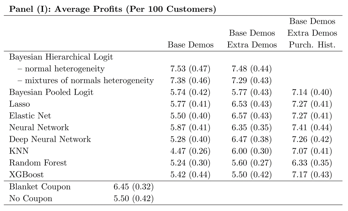
Used the degenerate strategies as benchmarks. What do you see?
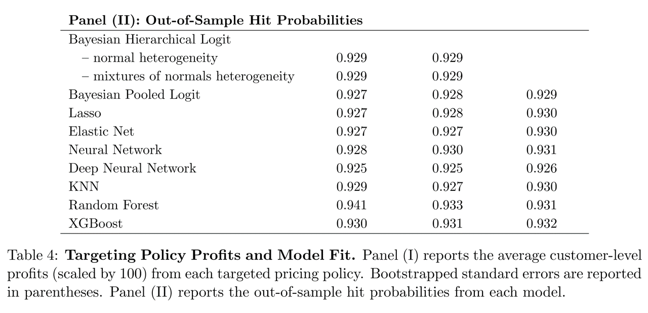
How did statistical criteria compare to economic criteria?
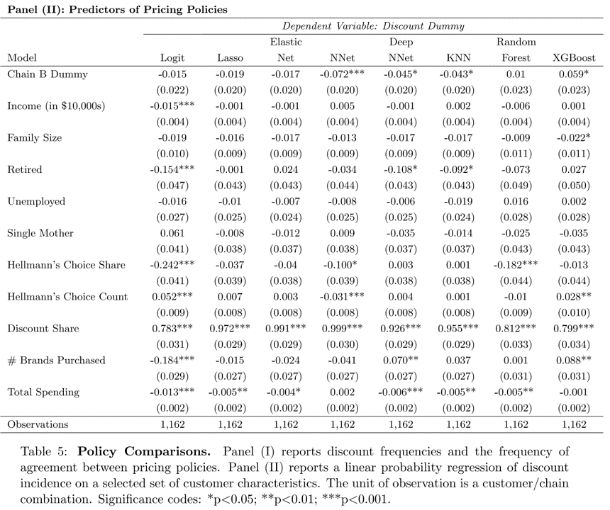
Past purchases on discount are, by far, the strongest predictor of models’ targeting decisions.
Takeaways
- To predict behavior, use past behavior
- Economic theory can help demand models to perform well with limited behavioral data
- ML model performance depends critically on data quality & abundance. Counterfactual predictions do not always outperform economic models
- Statistical performance \(\ne\) economic performance
Conjoint Analysis
- Generates stated-preference data to estimate heterogeneous demand model, to enable counterfactual predictions and optimal product designs and prices
- Probably the most popular quant marketing framework
Choosing Product Attributes
- Until now, we studied existing product attributes
- What about choosing new product attribute levels?
- Or what about introducing new products?
- Enter conjoint analysis: Attributes are Considered jointly
Survey and model to estimate attribute utilities- Autos, phones, hardware, durables
- Travel, hospitality, entertainment
- Professional services, transportation
- Consumer package goods
- Combines well with cost data to select optimal attributes
Conjoint extends demand modeling from “predict demand for existing products” to “predict demand for products that don’t exist yet.” When would a firm need this capability?
In cluttered categories, conjoint survey designs sometimes seek to replicate the experience of choosing from a typical product shelf. Should Red Bull be in its own refrigerator within the choice task?
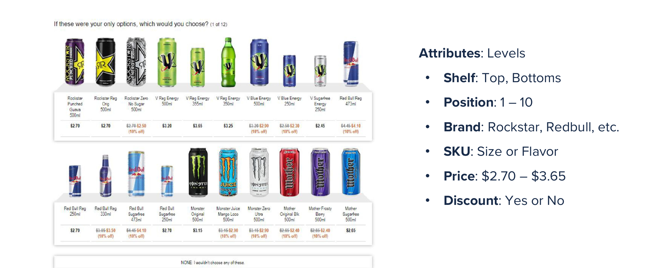
Sample Choice Task: Trucks

Conjoint respondents often have trouble deciding when choice tasks become too complex, so we usually limit stated-preference surveys to just a few product attributes. Then we use the stated-choice data to estimate heterogeneous \(\beta\) parameters for each level of each attribute.
Conjoint Analysis Algorithm
- Identify product attributes and levels/values : These constitute points in your attribute space
- Screen size: 5.5”, 6”, 6.5”, 7”
- Memory: 16 GB, 32 GB, 64 GB, 128 GB, 256 GB
- Price: $199, $399, $599, $799, $999
- Recruit consumer participants to make choices
- Recruit a representative sample of your target market
- Offer 8-15 choices among 3-5 hypothetical attribute bundles
- Sample from product space, record consumer choices
- Specify model, e.g. \(u_{jl}=x_{j}\beta_l-\alpha_l p_j+\epsilon_j\) and \(s_j=\frac{\sum_{l}x_{j}\beta_l-\alpha_l p_j}{\sum_l\sum_{k}x_{k}\beta_l-\alpha_l p_k}\)
- Estimate choice model
- Combine estimated model with projected cost data to choose product attributes and maximize profits
Let’s fill out a class conjoint about food at the ballpark; use code 920-89
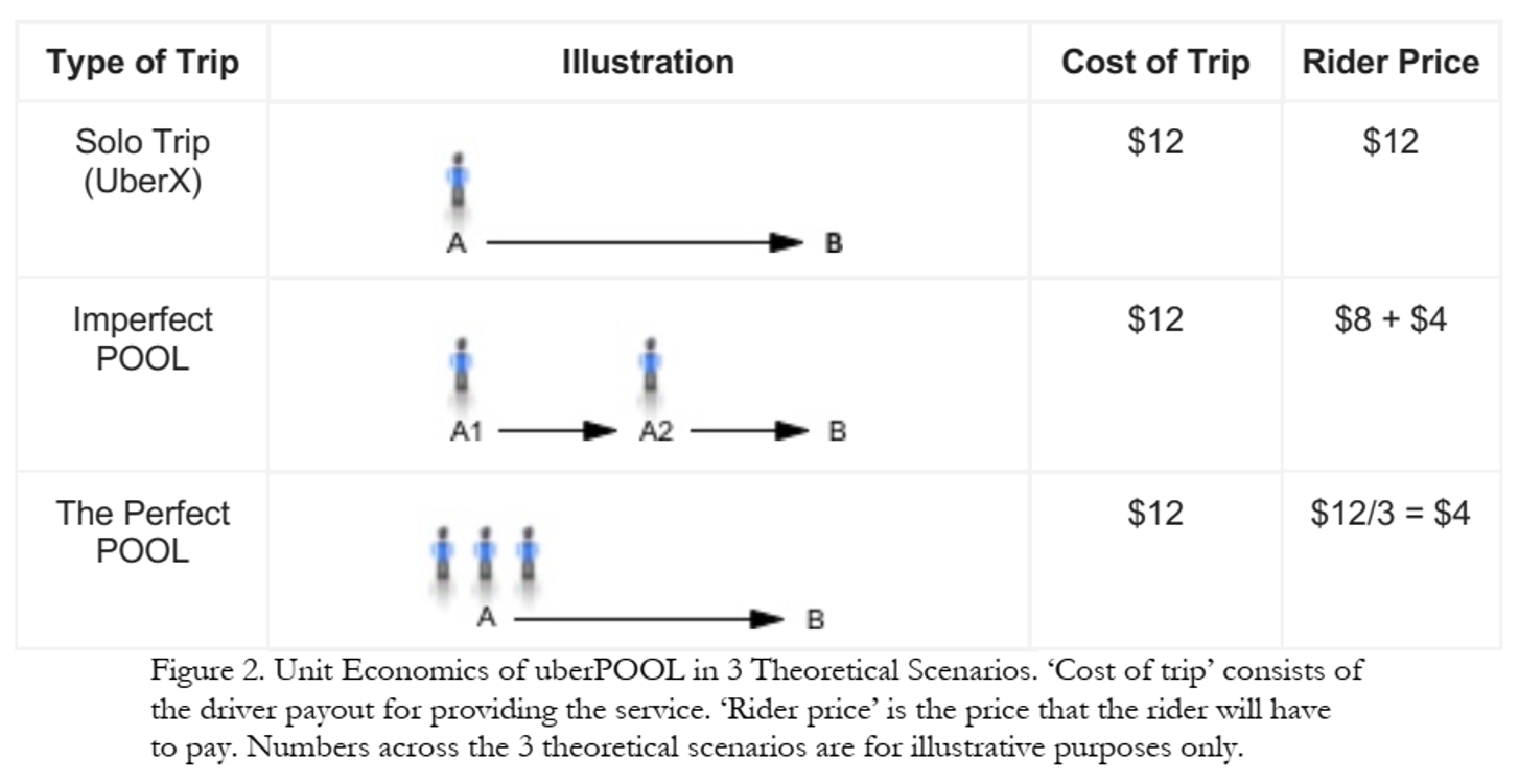
Case Study: UberPOOL
- In 2013, Uber hypothesized
- some riders would wait and walk for lower price
- some riders would trade pre-trip predictability for lower price
- shared ridership could ↓ average price and ↑ quantity
- more efficient use of drivers, cars, roads, fuel
Business Case Was Clear! But …
- Shared rides were new for Uber
- Rider/driver matching algo could reflect various tradeoffs
- POOL reduces routing and timing predictability
- Uber had little experience with price-sensitive segments
- What price tradeoffs would incentivize new behaviors?
- How much would POOL expand Uber usage vs cannibalize other services?
- Coordination costs were unknown
- “I will never take POOL when I need to be somewhere at a specific time”
- Would riders wait at designated pickup points?
- How would communicating costs upfront affect rider behavior?
Uber used Conjoint Analysis to design UberPOOL, so that key product attribute decisions could be informed by customer data.
Approach
- 23 in-home diverse interviews in Chicago and DC
- Interviewed {prospective, new, exp.} riders to (1) map rider’s regular travel, (2) explore decision factors and criteria, (3) a ride-along for context
- Findings identified 6 attributes for testing
- Online Maximum Differentiation Survey
- Selected participants based on city, Uber experience & product; N=3k, 22min
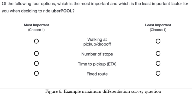
Open-ended interviews revealed key service attributes, then a forced-choice maxdiff measured which ones mattered most. How does this make the Conjoint survey more efficient?
Maxdiff Results

The Maxdiff results showed that walking and number of stops mattered less than arrival time, speed and duration. Do you think UberPOOL would be competing more with Uber or with public transit?
Conjoint Attribute Space
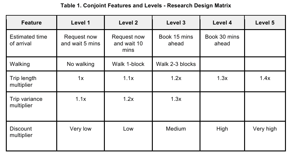
4 ETAs × 3 walking levels × 5 trip lengths × 3 variances × 5 discounts = 900 hypothetical services.
Conjoint Choice Task
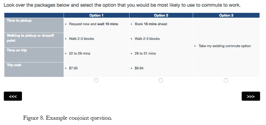
Each respondent saw 3 alternatives per choice task, and 7 choice tasks per respondent.
Heterogeneous Demand Model
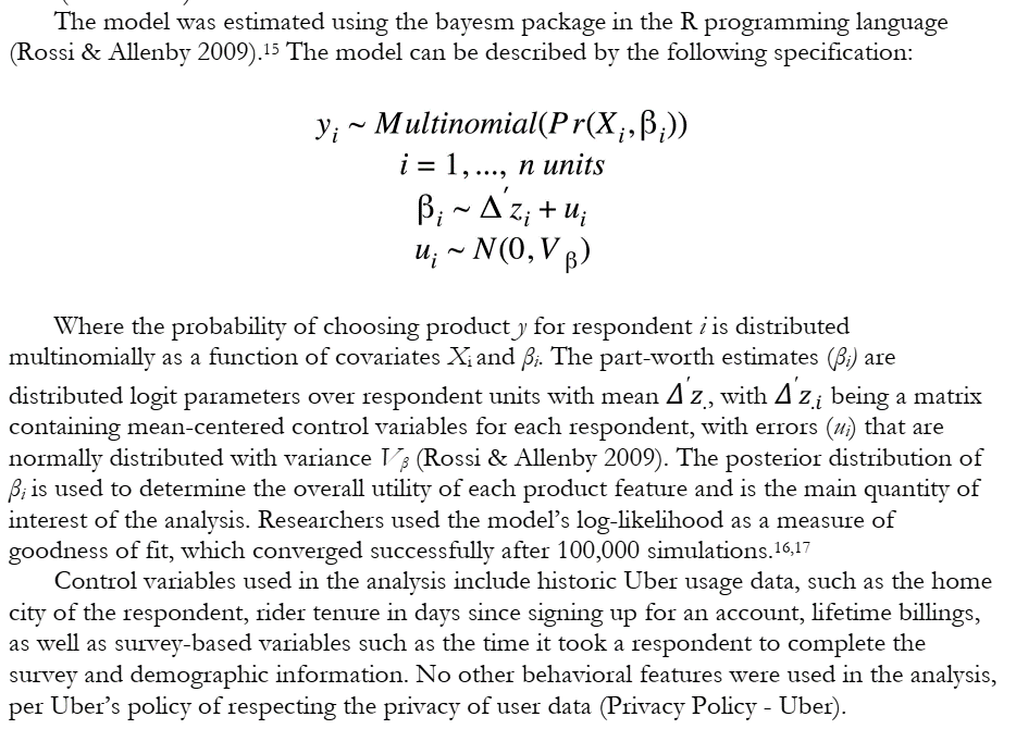
Uber invited 18k riders to complete 5-minute surveys, promising $500 Amazon gift cards to 5 respondents, leading to 1,934 survey completions at $1.29/survey. They used the data to estimate a heterogeneous MNL demand model.
Attribute Utility Estimates
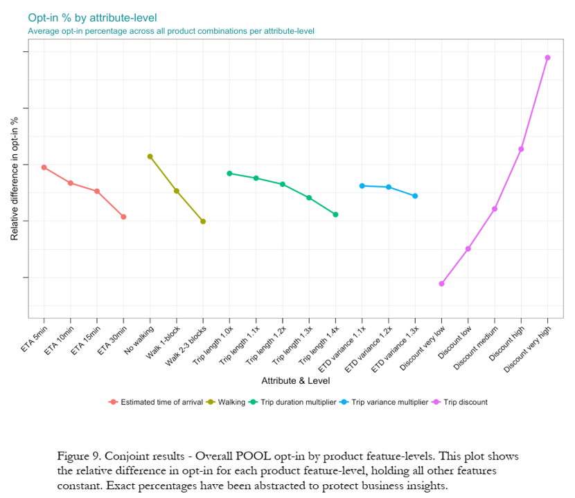
Y-axis labels held confidential, but slope = relative importance. Price matters most, by far. Trip variance doesn’t seem to matter much; how does this compare to Maxdiff results?
Business Results
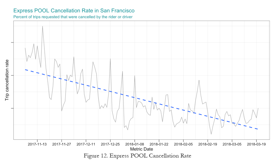
Product launch success was indicated by an initial match rate increase of 3.6%, higher shared trips, and declining cancellation rates over time. Profit impact was not disclosed.
Conjoint Pros and Cons
- Pro: It’s experimental, so we get causal effects by design. No endogeneity
- Pro: It’s purely hypothetical so we can test any scenario we can think of
- Pro: It’s fast and confidential, and relatively cheap
- Pro: Mature, competitive market of conjoint specialists
- Con: Requires representative sampling from target market
- Con: Relies on stated preferences: Participants need to imagine unfamiliar behaviors and report accurately; controlled environment will differ from real choice environment
Conjoint: Limitations, Workarounds
- We may fail to consider most important attributes or levels
- But we can consult with experts beforehand and ask participants during
- Additive utility model may miss interactions or other nonlinearities
- But this is testable & can be specified in the utility model
- Exploring a large attribute space gets expensive
- But we can prioritize attributes and use efficient, adaptive sampling algorithms
- Assumes accurate hypothetical choices based on attributes
- But we can train consumers how to mimic more organic choices
- Participants may not represent the market
- But we can measure & debias some dimensions of selection
- Stated preferences may not equal revealed preferences
- But we can model the retail channel, vary competing products, and perform conjoint regularly to evaluate predictive accuracy
- Participant fatigue or inattention; consumer preferences evolve
- But we can incentivize, limit choices, check for preference reversals, and repeat conjoints to gauge durability
Class Script
- Add heterogeneity to MNL model
- Cross-validation to compare models
Wrapping Up
Competition
- Use the class dataset. Find a new combination of customer attributes and product attributes that finds the demand model (
out_num) that maximizes thell_ratio(mdat1, out_num). - Evaluate your new demand model’s cross-validation performance using
cv_mspe(out_num, mdat1). - Use the
print()command to outputll_ratio(mdat1, out_num)andcv_mspe(out_num, mdat1)within your script.

Recap
- Understanding heterogeneous customer needs enables deep marketing insights (Quidel example)
- Demand models can incorporate discrete, continuous and/or individual-level heterogeneity structures
- Heterogeneity helps demand model fit better, but may predict worse past some point
- Conjoint analysis uses stated-preference data to map markets and predict profits of product locations in attribute space

Going Further
- Train (2009), Chapters 7-12
- Reconciling modern machine learning practice & the bias-variance trade-off
- MGT 108R to design & run conjoint analyses
- Conjoint literature is huge. Good entry points: Chapman 2015, Ben-Akiva et al 2019, Green 2022, Allenby et al. 2019
- Demand Estimation with Text and Image Data
- Advanced: Cal Tech Grad class on empirical IO